Pump System Curve Operating Head
Pump System Curve Operating Head
Every pumped piping system has its own "system curve" — the head the pump must supply at each flow rate — built from a flat static component plus a friction component that rises with the square of velocity. Where that curve crosses the pump's own head-flow curve is the actual operating point, so being able to write the system curve in closed form is the first step in any pump selection or troubleshooting exercise. A poorly estimated system curve is a classic cause of pump problems: oversizing the resistance term leads to a pump that never reaches its rated flow, while underestimating it can push the operating point into a region of poor efficiency or cavitation risk. This worksheet lumps all velocity-head and friction losses into a single empirical coefficient K so the curve can be evaluated directly at any flow.
The system head is H = H_static + K*Q^2, where the K term lumps all friction and minor losses. where H_static is the static lift (elevation plus any pressure head difference), K_sys is an empirical resistance coefficient carrying units of s^2/m^5 so the result comes out in metres, and Q_op is the operating flow rate.
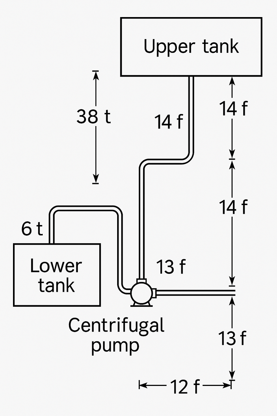
Inputs
H_static := 15 m=15 m
K_sys := 800 s^2/m^5=800 s^2/m^5
Q_op := 0.05 m^3/s=0.05 m^3/s
The resistance term scales with the square of flow, so doubling the flow quadruples the friction contribution — this is why the system curve bends upward sharply at high flow.
H_sys := H_static + K_sys·Q_op^2=17 m
Results
At low flow the system head approaches the static lift, while at high flow the K*Q^2 term dominates and the required head rises steeply — this is why throttling a valve (which raises K) moves the operating point to lower flow rather than higher. If a pump cannot reach the flow implied by intersecting its curve with this one, either the pump is undersized for the system or K has been underestimated, commonly from omitted fitting losses.
Assumptions & limitations
- K lumps pipe friction and all minor (fitting) losses into one constant.
- Assumes incompressible, steady flow with no elevation change during operation beyond H_static.
- K is only valid over the flow range it was fitted or calculated for.
- Does not include NPSH or cavitation checks on the suction side.