Mean and Standard Deviation of a Data Set
Mean and Standard Deviation of a Data Set
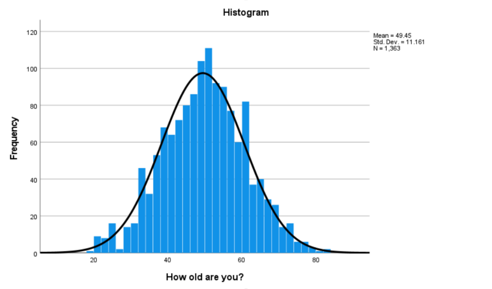
Summarizing a batch of measurements with a single "typical" value and a measure of scatter is one of the most common tasks in engineering and science — whether it is five tensile-test coupons, five temperature readings, or five days of production output. The mean locates the center of the data and the standard deviation quantifies how spread out the values are around that center.These two numbers underlie almost every downstream statistical decision: control charts, tolerance bands, and confidence intervals all start from a mean and a standard deviation. Computing them by hand from the defining sums (rather than a black-box function) makes clear exactly what "spread" means and why the denominator is n−1 for a sample rather than n.
The sample mean is the sum of the values divided by the count, and the sample standard deviation is the square root of the average squared deviation from that mean (using n−1 in the denominator). where x_1 through x_5 are the five sample values, mean_x is their average, var_x is the sample variance, and sd_x is the sample standard deviation.
Inputs
x_1 := 12=12
x_2 := 15=15
x_3 := 11=11
x_4 := 18=18
x_5 := 14=14
Add the five values and divide by the count to find the center of the data.
mean_x := (x_1+x_2+x_3+x_4+x_5)/5=14
Sum the squared distance of each point from the mean, then divide by n−1 (not n) — this "n−1" correction keeps the sample variance an unbiased estimate of the population variance.
var_x := ((x_1-mean_x)^2+(x_2-mean_x)^2+(x_3-mean_x)^2+(x_4-mean_x)^2+(x_5-mean_x)^2)/4=7.5
Taking the square root converts variance (squared units) back into the same units as the original data, giving a directly interpretable spread.
sd_x := sqrt(var_x)=2.74
Results
A standard deviation that is small relative to the mean indicates tightly clustered, repeatable data; here the spread is a modest fraction of the mean, typical of a well-controlled process. If sd_x were instead comparable in size to mean_x, that would flag high variability worth investigating before trusting the mean as representative. With only five points this estimate is itself noisy — more samples would tighten confidence in both statistics.
Assumptions & limitations
- Five independent, randomly sampled values.
- Sample (not population) standard deviation, n−1 divisor.
- No outlier rejection applied.
- Assumes the underlying distribution is reasonably well-behaved.