Matrices and vectors

Build the array with a constructor, give it a name, and every later region works on that name. Units ride along on the entries. A solved displacement vector comes back in millimetres, not as a bare column of numbers.

Write a matrix or a vector

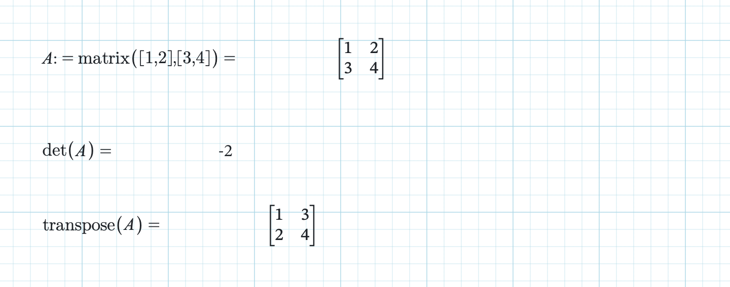
Each argument to matrix is one row, written as a bracketed list. Two brackets of two entries give a two-by-two:

A := matrix([1, 2], [3, 4]) =
B := matrix([1, 2, 3], [4, 5, 6], [7, 8, 10]) =
v := vec(1, 0, 0) =
I := eye(3) =
z := zeros(2, 2) =
x := linspace(0, 10, 11) =
r := range(1, 5) =

Bare scalars are each treated as a row of one, so matrix(1, 2, 3, 4) is a four-by-one column rather than a four-element row. Use vec when you want a vector. range(start, end) is inclusive at both ends, so range(1, 5) gives five values. rstep(start, next, end), which the ribbon labels 1,3..n, steps by next − start. Entries can carry units: matrix([1 m, 2 m], [3 m, 4 m]) keeps metres on the whole array.

On the ribbon, matrix is under Functions ▾ → Matrix alongside eigenvals and eigenvecs. Operators ▾ → Matrix is the operations palette rather than the constructors: a×b, ‖v‖, element access [i], M⊗ for kron, Mₙ for submatrix, M↺ for rotate, Mᵀ, range, 1,3..n, and V⃗ for vectorize. vec, eye, zeros, ones, diag and linspace have no button. Type them.

Linear algebra on a named array

• transpose(A) — the ribbon Mᵀ. tr(A) is the same function.
• det(A), inv(A) (M⁻¹), trace(A), rank(A).
• norm(v) (‖v‖), dot(a, b) (a·b), cross(a, b) (a×b).
• eigvals(A) and eigvecs(A), also spelled eigenvals and eigenvecs.
• shape(A) and size(A) when you need to check what you actually built.
• solve(A, b) for a linear system. That is a different thing from the Given-block solve.

A worked two-degree-of-freedom solve

Two 100 kN/m springs in series give the assembled stiffness matrix below. Load the first node with 10 kN and leave the second free:

K := matrix([200 kN/m, -100 kN/m], [-100 kN/m, 100 kN/m]) =
F := vec(10 kN, 0 kN) =
u := solve(K, F) =

u evaluates to 100 mm at both nodes. The grounded spring extends 100 mm under the 10 kN, and the second spring carries no force at all, so the free node just follows the first. You never wrote a unit for the answer: kN divided by kN/m is a length, and it comes back in millimetres on its own.

Vector work behaves the same way. With r := vec(0 m, 0.5 m, 0 m) and P := vec(2 kN, 0 kN, 0 kN), cross(r, P) gives −1 kN·m on the third axis, the moment of that force about the origin, while norm(vec(3 kN, 4 kN, 0 kN)) gives 5 kN as the resultant.

What units come back

Function	Unit of the answer
transpose, trace, norm, cumsum	Unchanged from the entries.
det	The entry unit raised to the power n for an n-by-n, so a two-by-two in kN/m gives a determinant in (kN/m)².
inv	The reciprocal of the entry unit.
dot, cross	The product of the two argument units.
solve(A, b)	The unit of b divided by the unit of A, reduced to base units.

Send an answer to a spreadsheet

Right-click a math region whose answer is a matrix and choose Export matrix to CSV…. The browser downloads a comma-separated file of the evaluated answer. The numbers, not the expression that produced them.

Names not covered here are in the function catalog. When the equations are nonlinear, or you cannot get them into matrix form at all, open a Given/solve block rather than reaching for solve(A, b).