Conditional formatting
A utilisation of 1.04 should announce itself. Right-click the region and set a rule. When the rule matches, the answer changes colour. The value itself does not change. The rules belong to that one region, not the whole sheet, and you reach them from the region's right-click menu, not from the ribbon.
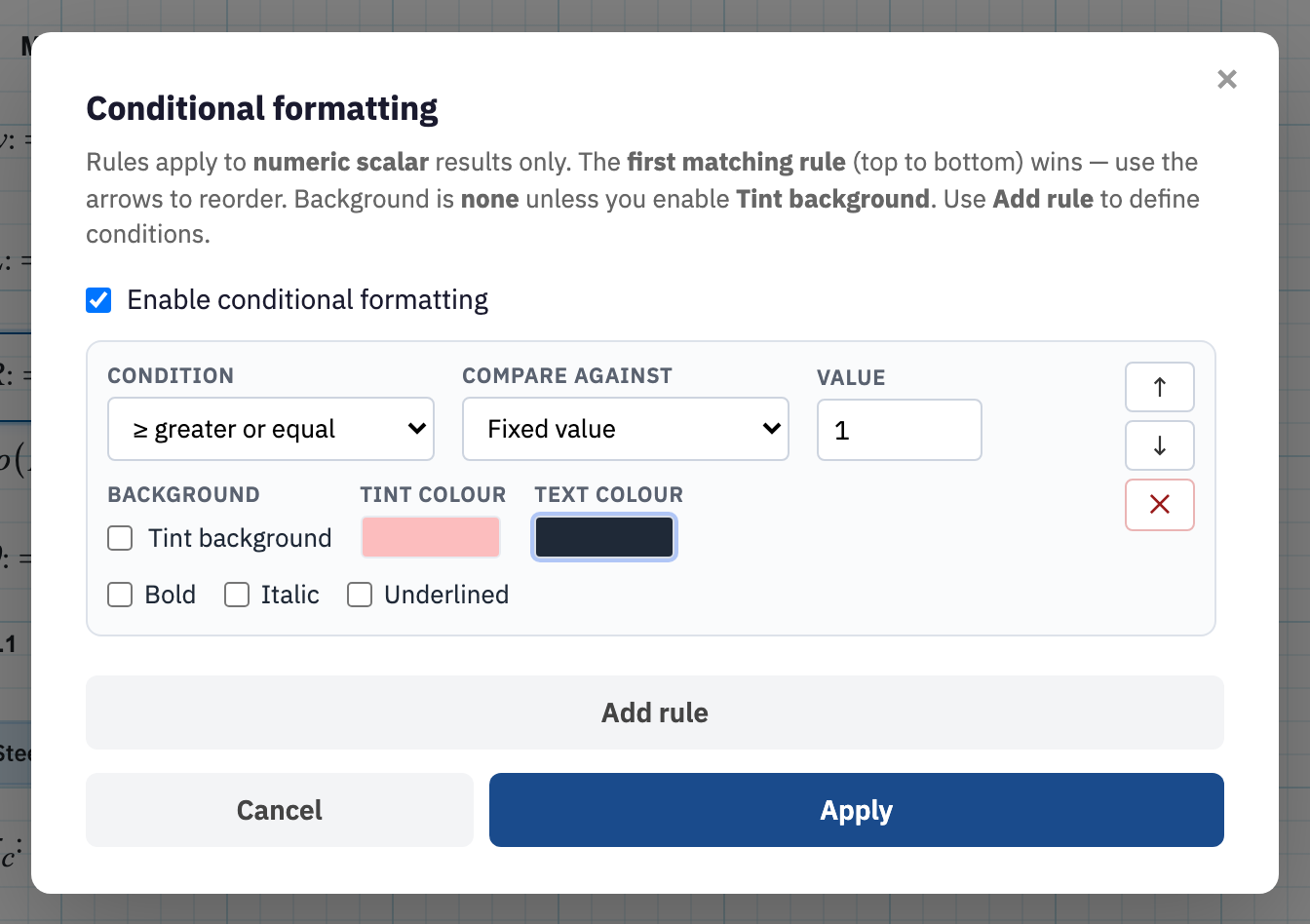
Set up the rules
- Right-click the math region and choose Edit conditional formatting…. The dialog is titled Conditional formatting.
- Tick Enable conditional formatting. Without this, saved rules sit dormant.
- Choose Add rule once per condition, and fill it in as below.
- Choose Apply to save. Cancel, the ×, or Escape discards. Clicking outside the dialog does not close it.
Two things the dialog's own help text is careful to say. Rules apply to numeric scalar answers only, and the first matching rule from the top down is the one that fires. Put your worst case first, or a broad rule will swallow the narrow one below it. Background is none unless you enable Tint background.
What a rule contains
- Condition — one of ≥ greater or equal, > greater than, ≤ less or equal, < less than, = equal, ≠ not equal.
- Compare against — either a Fixed value you type, or a Variable, meaning another name already on the sheet rather than this region's own assignment. Comparing against a variable keeps the limit and the check in step when the limit changes.
- Tint background is off by default. Turn it on to enable the Tint colour swatch beside it.
- Text colour is always available, as are Bold, Italic, and Underlined.
Each rule row carries ↑ and ↓ buttons to reorder it, which matters given first-match-wins, and ✕ to remove it. Copy the region and the rules come with it.
Turning rules off without losing them
Once rules are saved, the same context menu offers Disable conditional formatting or Enable conditional formatting, which is what you want before a plain black-and-white print. The rules stay defined either way, and Edit conditional formatting… still opens the full dialog.
A summary table that links to this variable inherits the same colours, so a pass/fail scheme set up once on the calculation carries through to the table you hand over.
Next, summary tables if you want those colours to carry through to a table you hand over.